Class 8: Slutsky Equation
Optional textbook reading: Varian, Chapter 8: “Slutsky Equation.”
Key Ideas
Last class ended with Ren, who packed more noodles when noodles got more expensive. Nothing about that violated the theory: Ren was choosing his favorite affordable bundle at every step. So the theory of demand, as it stands, allows demand to rise or fall when a price rises. That’s uncomfortable. Economists are confident that, with rare exceptions, an increase in price reduces the quantity demanded, and a theory that cannot account for why the exceptions are rare has limited explanatory content.
Today we sharpen the theory. The trick is to notice that a price change does two things at once. First, it changes the terms of trade: after coffee doubles in price, each cup now costs two units of everything else instead of one, so the consumer has a reason to swap coffee for other goods. Second, it changes purchasing power: the same $40 buys a smaller set of bundles than before, so the consumer is effectively poorer, and last class taught us that a poorer consumer buys less of a normal good but more of an inferior good.
The Slutsky decomposition separates these two channels. The part of the change in demand that comes from the new terms of trade is the substitution effect. The part that comes from the change in purchasing power is the income effect. The first problem today walks you through the mechanics.
The decomposition yields a clear prediction. The substitution effect always pushes demand against the price change. The income effect reinforces it for a normal good and fights it for an inferior good. So a Giffen good like Ren’s noodles has to be inferior, and inferior enough that the income effect swamps the substitution effect. Now we can explain why Giffen goods exist in theory but are almost never seen in practice.
Problems of the Day
Q25: Nothing Has Changed
Nadia spends her $40 weekly budget on fancy coffee (good 1) and everything else (good 2), and her utility function is \(u = x_1 x_2\). Both coffee and “everything else” cost $1 per unit. Then the café doubles coffee to $2, and Nadia’s office manager, feeling responsible (the café is his cousin’s), raises her weekly stipend by exactly enough that her old bundle is affordable again. “There,” he says. “Now nothing has changed for you.”
Find Nadia’s old bundle (call this A), the size of the raise, and what she actually buys after it (call this B). Was the manager right?
Now suppose there had been no raise. Find Nadia’s bundle in this case (call it C). We’ve finished the Slutsky decomposition of Nadia’s change in demand because of a change in the price of coffee. The idea is that when the price of coffee rose, Nadia changed her behavior for two reasons and two reasons only: she bought less coffee because it had become relatively more expensive (the substitution effect), and she bought less coffee because the price change made her, in effect, poorer (the income effect). Going from the amount of coffee in bundle A to B is her change in demand only because of the change in prices (not the change in purchasing power), so that’s the substitution effect. Going from the amount of coffee in bundle B to C is her change in demand only because of purchasing power, not because of the change in prices, so that’s the income effect.
What’s larger: Nadia’s substitution effect, or her income effect?
Q26: The Fare Hike
Dev has $36 a week to spend on bus rides (good 1) and everything else (good 2, $1 per unit). You are not told his utility function, only his demand for bus rides, \(x_1 = \dfrac{60 - m}{p_1}\), where \(m\) is his weekly budget. The fare is $2.
The transit authority announces a hike to $3. Councilmember Okafor objects: “Ridership will collapse.” Councilmember Reyes has a fix: “Then mail every rider a weekly voucher worth exactly enough to afford their old rides. Ridership won’t budge.”
Find Dev’s old bundle (A), the voucher he would need, what he buys with the hike and the voucher (B), and what he buys with the hike and no voucher (C). Compute the substitution and income effects. Who was closer to the truth? Reyes finds your answer for B baffling; explain it to her. What does the demand function tell you about bus rides for Dev, and does the sign of his income effect match the prediction in today’s Key Ideas?
Q27: The Painless Tax
Senator Vale unveils her plan on live TV: a $1 tax on every gallon of gasoline (currently $1 a gallon), with all the revenue collected pooled and mailed back to drivers in equal lump-sum rebates. “Gas use will fall,” she promises, “and since every dollar comes back, nobody ends up a dime worse off.”
Rosa has $30 a week to spend on gasoline (good 1, use \(p_1 = 1\)) and everything else (good 2, $1 per unit), and her preferences are \(u = x_1 x_2\). Assume the government keeps nothing and all drivers are alike. Find Rosa’s bundle before the plan, then after.
Is Senator Vale right: will gas use fall, and will nobody be made worse off?
Answers
Q25: Nothing Has Changed. With \(u = x_1 x_2\) Nadia spends half her income on each good, so \(x_1 = m/(2p_1)\) and \(x_2 = m/(2p_2)\). Before the price change, A \(= (20, 20)\). At the new prices that bundle costs \(2 \cdot 20 + 20 = 60\), so the raise is $20. With $60 she buys B \(= (15, 30)\). The manager is wrong: she drinks five fewer coffees and buys ten more units of everything else. In fact she is better off, not merely unharmed. Bundle A is still affordable and she chose B instead, so by revealed preference she prefers B; the utility numbers agree, \(450\) against \(400\). Making the old bundle exactly affordable always overcompensates, because the consumer can substitute away from the good that got expensive.
With no raise, C \(= (10, 20)\). The substitution effect, A to B, is \(15 - 20 = -5\) coffees. The income effect, B to C, is \(10 - 15 = -5\) coffees. The two effects are the same size here, and both push demand down, as they must for a normal good. In a diagram, B sits on a budget line with the new slope \(-2\) that passes through A, and C sits on the parallel line through the original income of $40.
Q26: The Fare Hike. At the old fare, A has \(x_1 = (60 - 36)/2 = 12\) rides and \(x_2 = 36 - 24 = 12\). The old rides cost \(12 \cdot 3 = 36\) at the new fare, so the voucher is \(12 \cdot (3 - 2) = \$12\), which raises his budget to \(m' = 48\). With the hike and the voucher, B has \(x_1 = (60 - 48)/3 = 4\) rides and \(x_2 = 48 - 12 = 36\). With the hike and no voucher, C has \(x_1 = (60 - 36)/3 = 8\) rides and \(x_2 = 36 - 24 = 12\).
The substitution effect, A to B, is \(4 - 12 = -8\) rides. The income effect, B to C, is \(8 - 4 = +4\) rides. The total effect is \(-4\): ridership falls from 12 to 8. Okafor has the direction right, though a one third drop is hardly a collapse. Reyes has it exactly backwards: her voucher cuts Dev’s riding to 4, half of what the hike alone would leave.
The explanation is in the demand function. Since \(x_1\) falls as \(m\) rises, bus rides are an inferior good for Dev. The voucher does nothing about the fact that a ride now costs three units of everything else instead of two, so the full substitution effect operates whether or not he is compensated. What the voucher adds is money, and a richer Dev rides the bus less. Equivalently, the hike without compensation makes him poorer, and a poorer Dev rides the bus more; that is why the income effect is positive here. The income effect fights the substitution effect, as the key ideas predict for an inferior good, but it is too small to win, so bus rides are inferior without being Giffen. One more thing worth noticing: in A and C he spends the same $12 on everything else. For this demand function \(x_2 = m - (60 - m) = 2m - 60\), which does not depend on the fare at all. Every change in the fare is absorbed entirely by his riding.
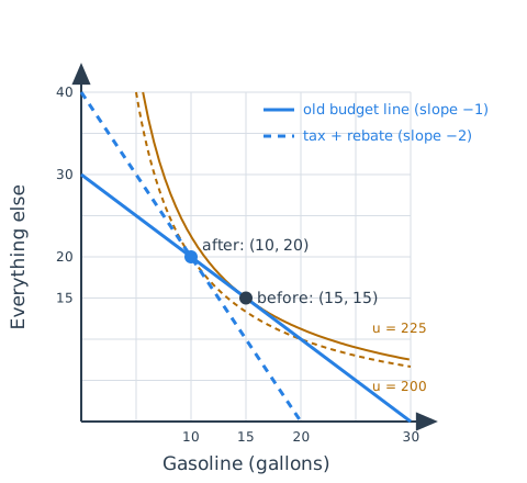
Q27: The Painless Tax. Before the plan Rosa has \(x_1 = 30/(2 \cdot 1) = 15\) gallons and \(x_2 = 15\). Under the plan gasoline costs $2 and Rosa, treating her rebate \(R\) as fixed, buys \(x_1 = (30 + R)/(2 \cdot 2) = (30 + R)/4\). The rebate is funded by the tax on what drivers actually buy, and all drivers are alike, so \(R = 1 \cdot x_1\). Solving \(x_1 = (30 + x_1)/4\) gives \(x_1 = 10\), hence \(R = 10\) and \(x_2 = (30 + 10)/2 = 20\). Her bundle under the plan is \((10, 20)\).
Vale is right about the first claim: gas use falls, from 15 gallons to 10. She is wrong about the second. The new bundle \((10, 20)\) costs \(10 + 20 = 30\) at the old prices, so it lies exactly on Rosa’s old budget line. This is no coincidence. Rosa pays \(t x_1\) in tax and receives \(t x_1\) back, so whatever she buys satisfies \(p_1 x_1 + x_2 = m\) at the pre-tax price. Now apply revealed preference: \((10, 20)\) was affordable before the plan, and Rosa chose \((15, 15)\) instead, so she likes \((15, 15)\) at least as well, and with strictly convex preferences strictly better. The utility numbers confirm it, \(225\) before against \(200\) after. Every dollar came back, and Rosa is still worse off.
The figure shows why. The tax-and-rebate budget line is steeper, with slope \(-2\), and it cuts the old budget line at the new bundle \((10, 20)\). Rosa’s best bundle on the steeper line is the point of tangency with \(u = 200\); her old bundle \((15, 15)\) is on the higher curve \(u = 225\), which the new line never reaches. The rebate restores her purchasing power in dollars, but the price she faces is distorted, and she gives up gallons she valued at more than they cost to produce.