Class 4: Utility
Key Ideas
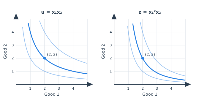
Last class you drew taste as a preference map: curves of bundles that tie, better bundles on higher curves. Today the curves get labels. A utility function is any formula that scores bundles so better always means bigger and ties score equal. The score works like elevation on a topographic map.
The analogy hides a trap. Elevation is a true quantity; 400 meters is twice 200. Utility is not. Only the order of the scores carries information: relabel every curve by any rule that keeps bigger bigger (double, square, etc.) and you describe the same preferences. Utility is ordinal, not cardinal.
Today we’ll explore:
- Which functions describe the same tastes?
- Which functions represent the preference maps from last class?
- How do you go from a function to a preference map?
Problems of the Day
Q11: The Grade Books
Professor Ferreira has taught the capstone course for twenty years. Each team submits a portfolio containing some number of lab studies (\(x_1\)) and some number of field reports (\(x_2\)), and every year she ranks the portfolios from strongest to weakest. The formula is simple: \(u = x_1 x_2\), so that a portfolio with 3 lab studies and 2 field reports gets a grade of 6, etc.
This year she is on sabbatical, and her three teaching assistants must run the grade book without her. Each proposes a new points formula to try:
- TA Amir, who worries that low scores discourage students: \(v = x_1 x_2 + 100\)
- TA Bea, who likes scores spread far apart: \(w = (x_1 x_2)^2\)
- TA Chen, who has always felt lab studies deserve extra weight: \(z = x_1^2 \, x_2\)
Score the portfolios (1, 2), (2, 1), (1, 4), and (3, 1) under all four formulas. Will any of the formulas always agree with Professor Ferreira’s in terms of ranking? Describe, as completely as you can, the entire family of grading formulas that never disagree with Professor Ferreira. You will have found what economists call the set of utility functions that represent the same preferences.
Under the professor’s formula, one portfolio scores 12 and another scores 4, and a student on the first team concludes: “ours is three times as good.” Under Bea’s formula those same portfolios score 144 and 16, which would make it nine times. Can both claims be right? Can either? State exactly which kinds of statements the numbers in a grade book can be trusted to make, and which kinds they cannot.
Economists play this exact game constantly, with a consumer in place of the professor and bundles of goods in place of portfolios. A formula that assigns a number to every bundle so that better always means bigger, and ties always mean equal, is called a utility function.
Q12: The Ghostwriter
Once you can draw someone’s preference map, you can go one step further and write their taste down as a formula. Your clients are the four customers you mapped in Q8: Priya, who only counts her total number of pens; Marco, whose left shoes are useless without matching right shoes; Dev, who likes pizza and would pay to avoid chores; and Sana, for whom more crackers are always better but exactly two pinches of salt is perfect.
Write a utility function for each of the four. Make sure to check each formula by picking two bundles that your Q8 map placed on the same indifference curve and confirm your formula gives them equal scores, then picking a bundle on a higher curve and confirm it scores strictly higher.
Q13: The Contour Plot
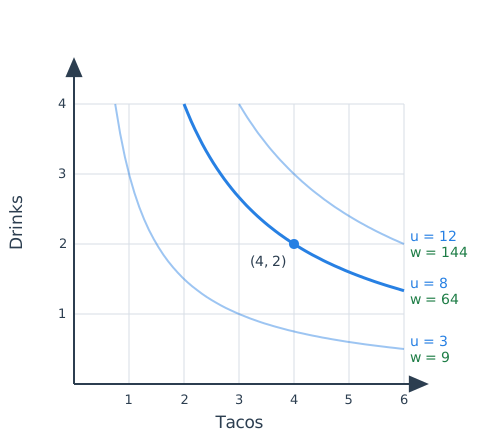
In Q8 you drew preference maps the hard way, by interviewing people about ties. Once a taste is written as a formula, the map comes free: an indifference curve is just a level curve of the utility function, the set of all bundles awarded one particular score. Mika spends her afternoons at the food trucks, and her taste for tacos (\(x_1\)) and drinks (\(x_2\)) is represented by \(u = x_1 x_2\).
Find every whole-number bundle that scores exactly 12, plot them all, and connect them into a smooth curve. Add the level curves for scores of 6 and 24, a few bundles each. Now read your drawing the way a hiker reads a topographic map. Which direction is uphill? Do the curves have the well-behaved shape from Class 3? And notice something the drawing is quietly telling you: can one of these curves ever touch an axis? (What score does a bundle with zero drinks receive, no matter how many tacos come with it?)
On your score-12 curve sit two extreme bundles, (1, 12) and (12, 1): a drink famine and a taco famine. Compute the score of their fifty-fifty mix. Do the same for the tamer pair (2, 6) and (6, 2). State what you find as a general rule about this taste, and then say it in plain language: what kind of eater does \(u = x_1 x_2\) describe? Now hunt for the exception: can you find any two bundles that tie under \(u\) whose fifty-fifty mix is not strictly better? What is special about your example? Finally, run the same experiment on Priya’s formula from Q12, \(u = x_1 + x_2\), and explain what the different outcome says about the link between bowed-in curves and a taste for mixing.
Answers
Q11: The Grade Books.
- The scores are:
| Portfolio | Ferreira \(u = x_1 x_2\) | Amir \(v = u + 100\) | Bea \(w = u^2\) | Chen \(z = x_1^2 x_2\) |
|---|---|---|---|---|
| (1, 2) | 2 | 102 | 4 | 2 |
| (2, 1) | 2 | 102 | 4 | 4 |
| (1, 4) | 4 | 104 | 16 | 4 |
| (3, 1) | 3 | 103 | 9 | 9 |
Amir and Bea reproduce the professor’s ranking exactly on these four, and in fact on every portfolio: \((1, 4)\) first, \((3, 1)\) second, \((1, 2)\) and \((2, 1)\) tied for last. Chen does not. He breaks the professor’s tie between \((1, 2)\) and \((2, 1)\), and he reverses her verdict on \((1, 4)\) versus \((3, 1)\), ranking the portfolio with three lab studies above the one with four field reports. That is no accident: his formula is a different opinion about what a strong portfolio looks like, which is precisely what he intended.
What Amir and Bea have in common is that each of their scores is computed from the professor’s score, and by a rule that never turns a bigger \(u\) into a smaller result. Adding 100 does that; squaring does too, as long as scores are never negative, which here they are not. The entire family of formulas that never disagree with Professor Ferreira is the set of all \(f(x_1 x_2)\) where \(f\) is a strictly increasing function: \(u + 100\), \(u^2\), \(\sqrt{u}\), \(\ln u\), \(5u - 3\), and infinitely many others. The converse also holds. Any formula that always agrees with her must give the same score to every pair of portfolios she ties, so it can only depend on the portfolio through \(u\); and it must give a higher score whenever she does, so that dependence must be increasing. Economists say that all of these formulas represent the same preferences. A utility function is never unique: once you have one, any increasing relabeling of it is just as good.
- Neither claim can be trusted, and the grade book itself shows why. Amir’s formula agrees with the professor on every ranking, and under it the two portfolios score 112 and 104, a ratio of about 1.08. If “three times as good” were a fact about the portfolios, two formulas that agree about every comparison could not disagree about it. The ratio is a fact about the formula, not about the work.
The same goes for differences. Ferreira’s scores differ by 8, Bea’s by 128, Amir’s by 8, and \(\sqrt{u}\) would make it about 1.46. What all the admissible formulas agree on is the order: which portfolio is stronger, and which portfolios tie. Those are the only statements the numbers can make. “Ours is better than theirs,” “those two are equally good,” and “ours beats theirs by more places in the ranking than it beats the third team” are safe. “Three times as good,” “twelve points better,” and “the gap between first and second is bigger than the gap between second and third” are not, because a harmless relabeling can change or even reverse them. Utility is ordinal: it ranks, and that is all it does.
Q12: The Ghostwriter. As in Q8, put the first-named good on the horizontal axis. Every answer below is one choice from an infinite family; any increasing relabeling of it describes the same client.
Priya. She counts pens, so \(u = x_1 + x_2\) with \(x_1\) blue pens and \(x_2\) black pens. Check: \((3, 1)\) and \((1, 3)\) both sat on her “four pens” line in Q8 and both score 4; \((3, 2)\) sits on a higher line and scores 5. A formula of the form \(ax_1 + bx_2\) always gives straight parallel contours; the slope \(-a/b\) is the rate at which the person will swap, and Priya’s is one for one.
Marco. His well-being is his number of matched pairs, which is the smaller of the two counts: \(u = \min(x_1, x_2)\) with \(x_1\) left shoes and \(x_2\) right shoes. Check: \((2, 3)\) and \((2, 5)\) both lie on the same L-shaped curve from Q8 and both score 2; \((3, 3)\) is the corner of the next curve out and scores 3. The \(\min\) is what makes the extra right shoes count for nothing.
Dev. Pizza is a good and chores are a bad, so the formula must rise in \(x_1\) (slices) and fall in \(x_2\) (hours): \(u = x_1 - x_2\) is the simplest. Check: \((4, 1)\) and \((5, 2)\) are on one of his upward-sloping curves, one slice compensating one hour, and both score 3; \((6, 1)\) scores 5. If your Q8 map used a different exchange rate, say two slices per hour, the matching formula is \(u = x_1 - 2x_2\). The minus sign is the whole point: a bad enters utility with the opposite sign from a good.
Sana. Salt is \(x_1\), crackers are \(x_2\). Crackers always help, and salt helps up to two pinches and hurts beyond, so the formula should reward being close to 2: \(u = x_2 - (x_1 - 2)^2\). Check: \((1, 5)\), \((3, 5)\), and \((2, 4)\) all score 4, and they do sit on one U-shaped curve, the first two on its arms and the third at its bottom; \((2, 5)\) sits on the next curve up and scores 5. The squared term is what produces the satiation point: it is zero at two pinches and grows in either direction.
The check in each case is the same: equal scores on one curve, strictly higher scores on a higher curve. A formula that passes it for every pair of bundles is a utility function for that client.
Q13: The Contour Plot.
- The whole-number bundles scoring 12 are \((1, 12)\), \((2, 6)\), \((3, 4)\), \((4, 3)\), \((6, 2)\), and \((12, 1)\). The curve through them is \(x_2 = 12/x_1\). For a score of 6 the bundles are \((1, 6)\), \((2, 3)\), \((3, 2)\), \((6, 1)\); for a score of 24 they include \((2, 12)\), \((3, 8)\), \((4, 6)\), \((6, 4)\), \((8, 3)\), \((12, 2)\).
Uphill is up and to the right: more tacos, more drinks, or both, always land on a higher curve. The curves slope downward and bow in toward the origin, so the taste is well-behaved in the Class 3 sense. The curves also never touch an axis. A bundle with zero drinks scores \(x_1 \times 0 = 0\) no matter how many tacos it contains, and the same is true of zero tacos, so both axes together form the score-zero “curve.” Every curve with a positive score stays strictly inside the quadrant: following \(x_2 = 12/x_1\) to the right, the curve flattens toward the taco axis forever without reaching it. In words, Mika will never give up her last drink for any number of tacos, and vice versa.
- The fifty-fifty mix of \((1, 12)\) and \((12, 1)\) is \((6.5, 6.5)\), which scores \(42.25\). The mix of \((2, 6)\) and \((6, 2)\) is \((4, 4)\), which scores 16. Both mixes beat 12, and the mix of the more extreme pair beats it by far more. The general rule is that the average of any two tied bundles scores strictly more than either, and the more lopsided the two bundles, the bigger the gain. In plain language, \(u = x_1 x_2\) describes someone who likes to mix: four tacos with four drinks beats twelve tacos with one drink, even though the second bundle has more items. Given a choice between two bundles she rates as equal, she would rather have half of each.
The exception has to be hunted for on the axes. Take \((3, 0)\) and \((7, 0)\): both score zero, so they tie, and their mix \((5, 0)\) also scores zero. No improvement. What is special is that the score-zero curve is not bowed at all: it is the two axes, which are straight lines, so the segment joining any two tied bundles on one axis lies entirely on the curve. Anywhere the curve is bowed, the segment joining two points on it passes strictly above the curve, into better territory. (The pair \((5, 0)\) and \((0, 5)\) does not work as an exception: their mix is \((2.5, 2.5)\), which scores \(6.25\), because the score-zero “curve” has a corner at the origin.)
For Priya, \((1, 12)\) and \((12, 1)\) both score 13, and so does their mix \((6.5, 6.5)\). The same is true of every pair of tied bundles, because her contour lines are straight: the midpoint of two points on a line is on that line. Mixing never helps her and never hurts her. The two experiments together say that the bow in an indifference curve is the taste for mixing. Strictly bowed-in curves mean averages beat extremes; straight-line curves mean averages merely tie extremes; and the only way averages could ever lose is for a curve to bow outward, away from the origin, which would be a person who prefers a famine of one good to a balanced meal.
Check Your Understanding
Utility and Ordinal Rankings
Writing Utility Functions
Cobb-Douglas Preferences
One family of formulas earns its own name: Cobb-Douglas utility functions have the form \(u = x_1^a x_2^b\), with positive exponents acting as weights on the two goods. Ferreira’s \(x_1 x_2\) and Chen’s \(x_1^2 x_2\) are both members. The family is popular because every member is well-behaved: curves slope down, bow toward the origin, and never touch an axis. And taking logs gives the relabeling \(a \ln x_1 + b \ln x_2\), the same preferences in additive form.